Motor control fundamentals

Telega performs field-oriented control of three-phase synchronous electric motors (referred to as “motor” from now on). This chapter provides a simplified overview of the main principles at the core of the motor control system. Knowing them is not necessary for deploying Telega but it helps achieve optimal performance.

Basic relations

This section introduces a few basic relations that are referenced in the subsequent description.

Voltage drop across an inductor: \(u = L \frac{di}{dt}\), where \(L\) is the inductance and \(i\) is the current over time \(t\).

Magnetic flux [weber] or [\(\text{tesla}\cdot\text{meter}^2\)]: \(\vec{\Phi} = \vec{B} A\), where \(B\) is the magnetic flux density [tesla] and \(A\) is the area. Also, see magnetomotive force (MMF).

Magnetic flux density [tesla]: \(\vec{B} = \vec{H}\mu\), where \(H\) is the magnetic field strength [\(\frac{\text{ampere}}{\text{meter}}\)] and \(\mu\) is the (absolute) magnetic permeability of the medium.

Strength of the magnetic field induced in a solenoid [\(\frac{\text{ampere}}{\text{meter}}\)]: \(\vec{H} = i\frac{n}{l}\), with the number of coil turns \(n\) and the axial coil length \(l\).

Magnetic flux linkage refers to some magnetic flux linking two bodies (e.g., a magnet and the coil of a solenoid). In a given flux-linked system, the part of the flux that does not participate in the linkage is the dissipation flux.

For a given solenoid (coil, electromagnet) \(\Phi \underset{\sim}{\propto} i\) for some small \(\Delta{}i\), all other things equal. With large current variations, the proportionality is not held due to permeability variation and core saturation.

The inductance of a given circuit relates to magnetic flux as \(L = \frac{\Phi}{i}\); therefore, \(\Phi = L \, i\). This relation is important as it gives rise to the dependency between the stator’s magnetic flux and its inductance, as will be shown later.

Mechanical power [watt] is a product of torque [\(\text{newton}\cdot{}\text{meter}\)] and angular velocity [\(\frac{\text{radian}}{\text{second}}\)]: \(P=\tau\omega\). By convention, the torque and the angular velocity have the same sign when the power is delivered from the motor to the load (this mode is called motoring); the signs are different when the power is absorbed from the load by the motor (this mode is called regenerative braking).

Root mean square (RMS) value of a sinewave is \(y_\text{RMS} = \frac{y_\text{amplitude}}{\sqrt{2}}\).

Motor construction

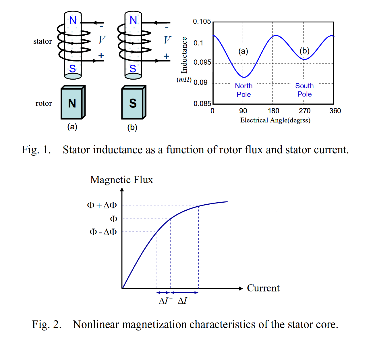
The motor consists of the stator and the rotor linked by a magnetic flux. The magnetic flux of the stator is excited by the stator coils, which are usually wound around the stator core; stator designs where the coil is air-cored are referred to as coreless. In synchronous three-phase motors, the magnetic flux of the rotor is either produced by permanent magnets, in which case the motor is referred to as a permanent magnet synchronous motor (PMSM), or by a dedicated excitation coil (which may be part of the rotor or part of the stator depending on the design), which is referred to as a separately excited motor. In the latter kind of motor, the rotor flux can be adjusted as necessary in real-time by changing the excitation current, but this process is slow, so from the standpoint of the vector control system, the rotor flux is assumed to be constant over a short time interval. The classification can be further refined but from the standpoint of motor control principles, there is little difference. The rest of this chapter applies to all of the listed types of motors unless specifically noted otherwise.

The number of magnetic poles of the stator is usually a multiple of three, while the rotor magnetic poles are usually even. The configuration of the motor’s magnetic system is conventionally denoted as \(xNyP\), where \(x\) is the number of stator poles and \(y\) is the number of rotor poles. The ratio of the pole counts cannot be arbitrary; in fact, there is only a small subset of valid configurations[1], such as 9N12P, 9N6P, 12N14P, 24N28P, 24N22P, 36N42P, etc. The ratio between the stator and rotor pole counts affects the cogging torque and some other properties of the motor to be covered later.

A motor with the elementary configuration of 3N2P will perform one revolution of the rotor per one period of the stator current; the mechanical ratio of such a motor is 1. Increasing the number of rotor poles will reduce the mechanical ratio, such that one mechanical revolution takes \(\frac{p}{2}\) periods of the stator current, where \(p\) is the rotor pole count. There is a derived concept of electrical angle, which refers to the phase of the stator current or the phase of the rotor within one electrical revolution, depending on the context. Since the power transfer performed by the motor is unaffected by the mechanical configuration, an increase in the pole count reduces the speed but increases the torque, all other things being equal.

In common iron-cored motors, part of the energy of the alternating stator current is unavoidably lost in the stator core (mostly in the form of eddy currents and remagnetization). The losses increase at higher current frequencies, i.e., at lower mechanical ratios or higher pole count values. On the other hand, a lower mechanical ratio enables lower stator currents at the same torque, which reduces resistive losses and possibly provides for a more efficient motor construction. The choice of the optimal magnetic system configuration is therefore highly dependent on the intended application of the drive and its typical operating conditions. In most practical applications concerned with energy efficiency, the frequency of the stator current does not exceed 1.5 kHz.

There are several key parameters characterizing a given motor aside from the magnetic configuration covered earlier. The phase resistance \(R_s\) [ohm] is the DC resistance of a single stator phase coil (the resistance between two phase wires is twice this value).

The phase inductance \(L\) [henry] is the inductance of the stator coil per single phase. Recall that the inductance of a solenoid is \(L = \frac{\mu \, n^2 \, A}{l}\), with \(n\) turns of wire across the axial length \(l\) with the cross-sectional area \(A\), and \(\mu\) is the magnetic permeability of the core (n.b.: reluctance is inversely proportional to permeability for a given geometry). The permeability of the magnetic circuit of a given phase changes depending on the angular position of the rotor and the direction and magnitude of the phase current, which alter the inductance of that phase, which in turn gives rise to certain important effects that are reviewed later. Due to changes in the inductance, the magnetic flux excited by the stator as a function of current is also variable, since \(\Phi = L \, i\).

The flux linkage \(\phi\) [weber] is the magnitude of the magnetic flux linking the rotor poles (e.g., permanent magnets in the case of PMSM) with the winding of the stator coil. For PMSM motors, this parameter is determined by the number of magnets, their magnetization, the number of turns in the stator coil, and the geometry of the rotor and the stator. For separately excited motors, this parameter is controlled by changing the current through the excitation coil.

A rotor pole moving next to a stator arm induces an electromotive force (EMF) in the latter’s coil (commonly referred to as back-EMF due to its origin being the motor rather than any external source). As the pole moves on and its opposite counterpart takes its place, the direction of the electromotive force is reversed. The EMF induced in the motor thus follows a periodic pattern aligned with the motion of the rotor. The amplitude of the back-EMF is a product of the electrical angular velocity and the flux linkage. If the flux linkage is independent of the angular position of the motor, the EMF follows a sinusoidal pattern, which is the case in most high-power motors. Smaller lower-power motors, commonly used in robotic applications and unmanned vehicles, are usually constructed such that the flux linkage changes depending on the angular position of the rotor (as it simplifies the motor construction). The resulting EMF changes in a distorted pattern that somewhat approximates a trapezoidal waveform. The oscillograms below show the trapezoidal EMF waveforms obtained by measuring the phase voltages relative to their midpoint while rotating the motor shaft externally:

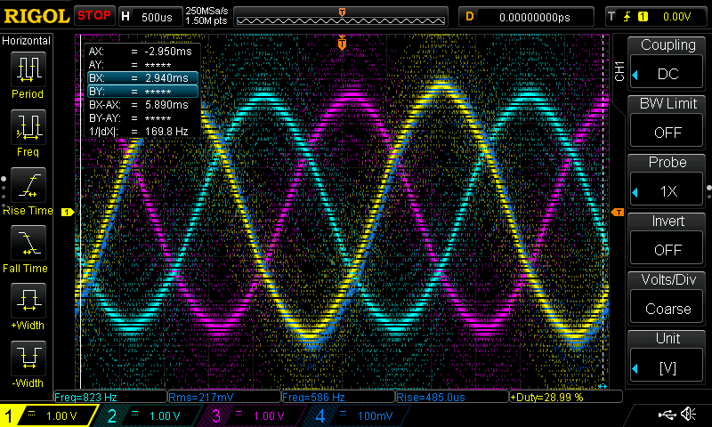
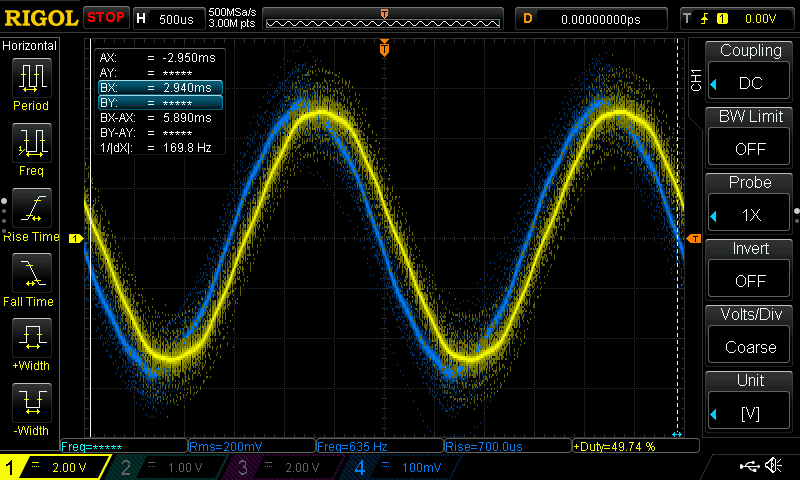
On the first oscillogram, channels 1, 2, and 3 display the phase voltages A, B, and C, while channel 4 displays the phase A current through a resistive load. The variable flux linkage of this motor can be observed by noticing the long parallel sections of the EMF waveforms. This effect can be amplified by measuring the voltage difference between any two phases, as shown on the second oscillogram, where channel 1 shows the A-B voltage difference.

The following discussion assumes an ideal motor with position-independent flux linkage (sinusoidal EMF). If this assumption does not hold, the deviations caused by the flux linkage variation are perceived by the control system as noise and are suppressed.

The amplitude of the back-EMF is \(u_\text{BEMF} = \phi \, \omega_e\), where \(\omega_e\) is the electrical angular velocity in \(\frac{\text{radian}}{\text{second}}\); recall that it relates to the motor angular velocity as \(\omega_e = \omega \frac{p}{2}\). One closely related parameter commonly used in the industry is the motor speed constant aka \(K_V\), which is defined as \(K_V = \frac{20 \sqrt{3}}{\pi \, p \, \phi}\); the unit is \(\frac{\text{RPM}}{\text{volt}}\) (\(p\) is the number of rotor poles)[2]; the physical meaning is the angular velocity of the motor in revolutions per minute required to excite the rectified EMF of 1 volt. Solve for \(\phi\) to obtain the flux linkage from \(K_V\): \(\phi = \frac{20 \sqrt{3}}{\pi \, p \, K_V}\).

The flux linkage can be easily measured by rotating the motor shaft and observing the phase voltage amplitude and its frequency (the phase voltage is the difference between the voltage of any phase and the zero voltage; the zero can be obtained with a high-resistance Y-bridge connected between the three phases):

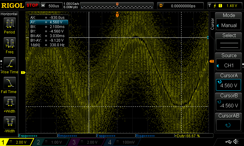
Deducing the flux linkage by measuring the frequency and amplitude of the back-EMF

As seen on the oscillogram, the phase voltage has an amplitude of 4.6 V and frequency of 330 Hz. The electrical angular velocity is frequency multiplied with \(2\pi\): 2073 rad/s. From this, we obtain the flux linkage value as \(\frac{u}{\omega_e}=2.22\) milliweber. The rotor pole count for this motor is 42, hence \(K_V=118\). The \(K_V\) value reported by the manufacturer for this motor is 120, which is reasonably close.

As mentioned earlier, the inductance of the stator phase winding changes depending on the angular position of the rotor, the magnitude of the phase current, and its direction. The former effect (position dependence) arises from the fact that the magnetic circuit is closed through the rotor whose reluctance (and permeability) is non-isotropic. The dependency on the current magnitude is due to the changes in the permeability of the stator core with the strength of the magnetic field; the magnetic field strength is proportional to the current:

Variation of the magnetic permeability with the strength of the magnetic field.

As we know from the inductance equation introduced earlier, it is linearly dependent on the permeability of the core. The dependency of the inductance on the direction of the current is also related to the permeability variance. As seen from the plot above, permeability is a function of the magnetic field strength \(H\); given the same stator current, permeability would be different depending on whether the magnetic field of the rotor pole is aligned or counter-aligned with that of the stator arm. This is illustrated in the following diagram:

Source: “A New Sensorless Starting Method for Brushless DC Motors without Reversing Rotation”, Yen-Chuan Chang and Ying-Yu Tzou.

The flux equation suggests that the stator flux is also dependent on its permeability. As permeability changes with the magnetic field strength, the resulting dependency of the stator flux on the stator current is non-linear, especially at high current amplitudes.

The position-dependent inductance variability is, by far, the most significant for most applications. It can be observed directly with an LCR meter connected with one probe to one phase and the other probe to the other two phases (shorted together). As the rotor is slowly rotated (not faster than approx. one revolution per minute; this can be done by hand), the reading would change between the minimum and the maximum:

The rotation has to be very slow or intermittent to avoid the induced EMF from distorting the voltage drop measurements performed by the instrument. For most motors, the phase inductance is at the lowest when the rotor pole is aligned with the stator pole, and at the highest when the rotor pole is halfway between the stator poles. As will be shown later, the former case (aligned) is referred to as direct axis (D-axis) alignment, and the latter case is quadrature axis (Q-axis) alignment. These respective inductances are referred to as \(L_d\) and \(L_q\). Note though that the values obtained from the LCR meter are those of one phase connected in series with the other two phases in parallel, so the measured value should be divided by 1.5.

Zubax Robotics maintains a publicly accessible spreadsheet that lists the key parameters of some of the popular motor types frequently encountered in the field: https://docs.google.com/spreadsheets/d/1Is3rCVp-Ibe1MELjCmrP3yA8ozJ6n9Sme-N9w2nRsi0.

Coordinate frames and transformations

In this section, we assume that the motor configuration is the elementary configuration, 3N2P: each phase has one stator arm and the rotor has one south pole and one north pole. From the standpoint of the electromagnetic system of the motor, all other magnetic configurations can be trivially reduced to the elementary configuration.

The rotor is said to be aligned with the stator when the magnetic flux vector of the rotor is co-directed with the magnetic flux vector of the stator. As long as the alignment is maintained, the torque is zero; conversely, the torque is maximized when the misalignment approaches 90°. Since the torque is dependent on the stator current (nearly proportional under some fixed rotor angle and small \(\Delta{}i\)), it follows that optimal control requires the angle between the magnetic flux vectors of the rotor and the stator to stay near 90°.

To simplify one’s reasoning about the magnetic system and its vectors, several trivial geometric transformations are applied. Here, we operate on a 2D plane, where the motor is projected such that its axis is perpendicular to the plane.

The magnetic flux vector of the stator is a product of the three-phase currents A, B, and C. This three-phase system is a balanced one, meaning \(0=A+B+C\). 2D vector manipulation in this ABC system is inconvenient due to its inherent redundancy; hence, a trivial geometric transformation that maps the ABC components onto a new \(\alpha\beta\)-frame, where A is projected onto \(\alpha\), and the \(\beta\)-projection is a function of B and C, is applied. This transformation is known as \(\alpha\beta\)-transformation, aka Clarke transformation.

Since the objective of vector control is to orient the magnetic flux vector of the stator relative to the position of the rotor, it is convenient to introduce an additional coordinate frame that is attached to the rotor, otherwise known as the rotating frame. It is still possible to solve the problem within the \(\alpha\beta\) frame (aka stationary frame) but it would make the formulation unnecessarily involved. The rotating frame is composed of axes \(d\) and \(q\), where \(d\) is co-directed with the north pole of the rotor (n.b.: co-directed with its magnetic moment vector) and \(q\) complements it. The axes are also commonly referred to as direct and quadrature, respectively. The mapping from the stationary \(\alpha\beta\) frame to the rotating \(dq\) frame is performed by the \(dq\)-transformation, aka Park transformation; it is dependent on the angular position of the rotor.

The magnetic flux \(\Phi\) excited by the stator is a function of the current, the stator coil geometry, and the magnetic permeability of the circuit. Assuming the geometry and the magnetic properties of the stator are constant, we have \(\vec{\Phi} \underset{\sim}{\propto} \vec{i}\). Therefore, assuming that the magnetic properties are known, control of the stator flux \(\vec{\Phi}\) is performed by controlling the stator current vector \(\vec{i}\). Non-linear effects caused by the magnetic permeability variance and magnetic saturation complicate the system but the general principles stand.

The diagram shows the \(\alpha\beta\) frame attached to the stator (notice how \(\alpha\) is aligned with phase A and \(\beta\) is on the same semi-plane with phase B) and the \(dq\) frame attached to the rotor (notice how axis \(d\) is aligned with the north pole of the rotor). The forward torque is created when the q-axis projection of the stator current vector \(\vec{i}\) is positive; in this diagram, this would result in counter-clockwise torque. The angular position of the rotor \(\theta\) on this diagram is 135°.

Synchronous motor coordinate frames

As the d-axis flux is excited by the rotor (either by its magnets or by the separate excitation coil), in the ideal case, the stator flux can be kept strictly at 90° for optimal control. If the projection of the stator flux onto the d-axis is non-zero, the flux of the rotor changes accordingly since the two are summed. In PMSM motors, this effect can be leveraged to adjust the rotor flux dynamically as needed by simply rotating the stator flux vector (in separately excited motors, this is normally redundant since the same effect can be achieved by reducing the rotor excitation current). While increasing the rotor flux serves little practical purpose in most applications (flux strengthening is rarely applied), its reduction can be useful during high-speed operation as will be reviewed below; this operating mode is known as flux weakening.

Vector control system

The vector control system updates its state periodically. Each update is referred to as a tick; the update interval is therefore the tick period. The control system may change the tick period at runtime dynamically to optimize its performance and minimize the energy consumption of the drive.

The control system is cascaded, where the bottom layers are responsible for the low-level motor torque and motion management while the top layers are closely involved with the specifics of the application at hand. The bottom layers are shared irrespective of the business objective because the principles of motor control are virtually invariant to the application of the motor, while the top layers are plugged as necessary (e.g., regular traction drive mode, servo mode, etc). This section is focused on the bottom layers.

The motor is connected to the three-phase voltage source inverter (VSI) equipped with the voltage and current feedback for each phase:

Simplified voltage source inverter (VSI) schematic

The VSI driver receives phase voltage setpoints from the higher-level control cascades. Since the control objective for the bottom layers is not the voltage but the stator currents, current controllers are introduced that generate voltage commands based on the target current values and the phase current feedback from the sensors. The current controllers are mostly tuned automatically by the control system based on the known motor parameters, but the user is provided with one dimensionless scalar parameter known as the bandwidth ratio (BWR) for trading off the responsiveness against noise resilience.

The command for the current controllers is generated by the torque & flux controller, which in turn accepts the desired torque command from the higher layers of the control system (e.g., velocity controller) which are not reviewed in this section. Optionally, the vector control system can be put into a special low-level operating mode where the torque & flux controller is bypassed, enabling direct control of the Q-axis voltage. The purpose of this control mode is to emulate the response of simple trapezoidal six-step controllers commonly found in some simple applications.

The vector control system can operate either in sensored or sensorless mode. In the sensored mode, an external rotor position sensor is introduced, whose readings are fed into the state estimator along with the phase current and voltage measurements \(\vec{i}_{abc}, \vec{u}_{abc}\). In the sensorless mode, the required information is deduced from the currents and voltages alone using some non-linear state estimator such as the constrained extended Kalman filter.

The vector control system provides feedback to the higher control layers, which includes rotor position \(\theta\), angular velocity \(\omega\), and torque \(\tau\). Internally, the electrical angle \(\theta_e\) is leveraged for \(dq\) (aka Park) transformations; the electrical angle is estimated separately and no assumptions concerning the relation between the mechanical and electrical angles are made.

The resulting structure is shown in the following diagram:

Synchronous vector control structure

The space vector (SV) voltage modulator is responsible for computing the individual phase voltage commands for the VSI from the \(\vec{u}_{\alpha\beta}\) command vector. The voltage modulator can switch between different modulation strategies depending on the current operating conditions to minimize energy losses in the system. An example where changing the strategy allows the drive to modulate higher-amplitude phase voltage is shown below: on the left, the phase voltages follow the naive sinewave, and on the right, a more sophisticated vector strategy is used where the zero point (the midpoint) is shifted to maximize the voltage utilization (n.b.: \(\sqrt{2}\approx{}1.41\)):

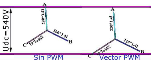
Phase voltage modulation strategies. The original illustration is made by Max La and published under CC BY-SA 3.0.

The following diagram (from SITL simulation) shows the voltage waveforms around the modulation switch point which occurs when the DC link voltage is exhausted; notice that there are separate voltage waveforms provided: A, B, and C referenced to the DC link ground (as seen by the VSI), and the same three phases referenced to their floating midpoint (as seen by the motor):

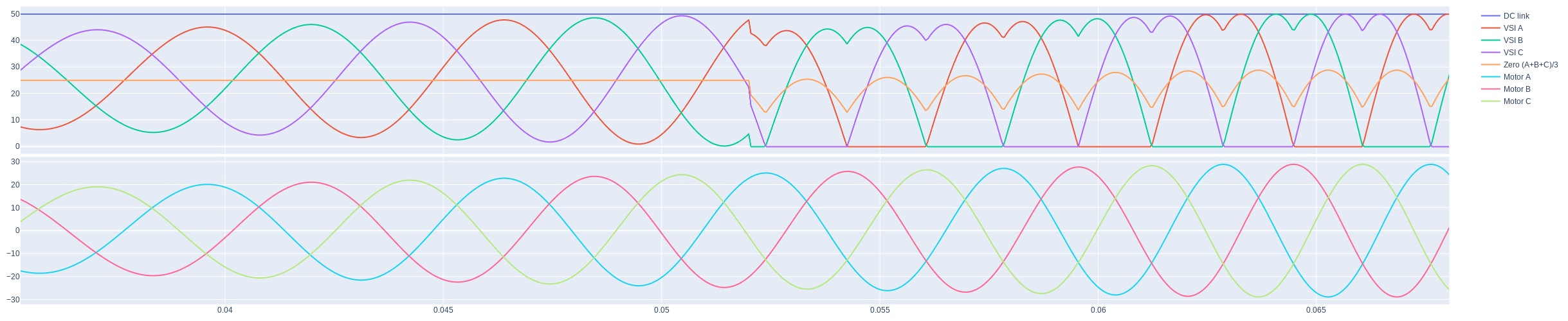
VSI modulation strategy switching

The sinewave modulation shown on the left is evidently unable to fully utilize the DC link voltage. The more sophisticated modulation shown on the right is one of many possible voltage-optimal modulation strategies. The maximum amplitude attainable with a voltage-optimal modulation strategy for a given DC link voltage is \(u_\text{max} = f_\text{util}\frac{u_\text{dc}}{\sqrt{3}}\), where \(f_\text{util} \leq 1\) is a dimensionless voltage utilization factor that accounts for the limitations of the VSI circuitry. The specifics are outside the scope of this general overview but the two most common causes for \(f_\text{util}<1\) are the limitations of high-side bootstrap transistor drivers and low-side current shunts.

From the definition of the \(\alpha\beta\) and \(dq\) transforms, it follows that \(\sqrt{u_d^2 + u_q^2} \leq u_\text{max}\). This effectively defines the power limit imposed by the DC link supply voltage. In certain applications, increase of the voltage utilization through clipping may be feasible; this results in distorted voltage waveforms as shown below.

Voltage clipping results in voltage waveform distortion

The torque & flux controller is responsible for computing the quadrature current component \(i_q\) required to deliver the requested torque at the shaft, and the direct current \(i_d\) required to manage the rotor flux. The basic torque equation is \(\tau = \frac{3}{2} \frac{p}{2} i_q \left[\phi + (i_d (L_d - L_q)) \right]\); the term \(i_d (L_d - L_q)\) is low in highly isotropic rotors where \(L_d \approx L_q \implies \Phi_{d,\text{stator}} \approx \Phi_{q,\text{stator}}\). This relation does not reflect certain complex non-linear effects such as core saturation. Management of the rotor flux is mostly focused on the flux weakening mode introduced earlier and the so-called maximum-torque-per-ampere (MTPA) current trajectory.

A simplified state equation of the motor expressed in the rotating \(dq\) frame is as follows:

\[\begin{split} \begin{align} \phi_d &= L_d i_d + \phi \\ \phi_q &= L_q i_q \\ u_d &= R_s i_d + \frac{d\phi_d}{dt} - \omega_e \phi_q \\ u_q &= R_s i_q + \frac{d\phi_q}{dt} + \omega_e \phi_d \end{align} \end{split}\]

Where \(R_s\) – stator phase resistance (half of phase-to-phase resistance) [ohm]; \(L_d,L_q\) – phase inductance when the rotor is aligned along the direct and quadrature axis, respectively [henry]; \(\phi\) – flux linkage [weber]. Projection of the flux linkage upon the \(dq\) frame is denoted as \(\phi_d,\phi_q\). Note that \(L \frac{di}{dt} = \frac{d\phi}{dt}\); under steady-state conditions this term is zero.

From the definition of \(\phi_d\), the principles of basic flux weakening operation become apparent: supplying some \(i_d < 0\), it is possible to partially suppress the rotor flux and thus increase \(\omega\) while keeping \(|u_{dq}|\) constant.

Internally, the state estimator maintains a model of the motor based on a similar state equation with additional provisions for certain more complex non-linear effects. The model is subjected to the same conditions and influences as the real motor, which are assessed using the phase current/voltage sensors and, optionally, the rotor position sensor; then the state of the model is updated based on its expected response. The state of the model is then used in place of the state of the motor.

The model of the motor is imperfect and the feedback from the sensors is imprecise, which introduces unavoidable divergence between the state of the real motor and the model maintained by the state estimator. All three of the estimated states (\(\theta,\omega,\tau\)) are closely linked but the most critical for the control system is the angular position \(\theta\) (as seen from the dq-transformation). The system can retain stability as long as the angle error is small, thanks to the negative feedback formed through the rotor flux variation. The following diagram shows two divergent coordinate frames: the real dq-frame attached to the motor \(d_r q_r\), and the estimated dq-frame attached to the model \(d_e q_e\); the estimated frame leads the real frame by \(\theta_\text{error}=+15^\circ\):

DQ system angle error

In the pictured configuration, the quadrature-axis current is positive (therefore, the torque is positive, which is the normal motoring mode); the direct-axis current is slightly negative, hence the direct-axis stator flux is also slightly negative. Due to the positive angle error, the projection of the stator flux onto the real d-axis is greater in magnitude than its modeled counterpart; observe \(i_{dr} < i_{de}\). This results in rotor flux weakening that is not accounted for by the state estimator. The weakened flux results in the \(\phi_d\) term, in the state equation above, exceeding the actual flux magnitude, which leads the state estimator to predict a lower angular velocity \(\omega_{ee} < \omega_{er}\). The same principle applies in the opposite case where the rotor flux is strengthened. As the sign of the angular velocity estimation error induced by the unaccounted flux adjustment is always opposite to the angle error, the angle error will eventually converge to a small value.

The above-described equilibrium is dependent on \(i_q\geq{}0\). Observe that when \(i_q<0\), the feedback loop closed through the rotor flux becomes positive, which creates complications for the state estimator in the sensorless mode. This is why sensorless vector control drives often have to limit the maximum braking torque (or, in other words, limit the minimum \(i_q<0\)), aside from other measures (which are typically either protected as key IP or are patented).

Imperfection of the model and distortions in the sensor feedback cause the estimator to always mispredict the motor state, but as long as the error is low, the system is able to retain stability. In a real drive, the error constantly changes as the drive is subjected to different operating conditions, such as abrupt load variation, steep acceleration, heating, etc. Even if the estimation error does not affect stability in a given application, it may significantly affect the energy efficiency of the drive, because angle estimation error invariably results in the stator energy being wasted on unnecessary flux adjustment and increased reactive power. A basic rule of thumb one can rely on is that a drive that is stable under abrupt load variation and during steep acceleration/deceleration is unlikely to incur a large static angle error estimation (otherwise, it would not be stable), and therefore, its energy loss is likely to be minimized. This is particularly important for sensorless drives.

The state equation allows one to infer the influence of each parameter on the performance of the drive:

• The influence of the flux linkage is the most prominent at high angular velocities.

• The inductances are especially significant in the presence of steep current gradients.

• The resistance is critical under load.

These simplified relations allow one to assess the correctness of the motor parameters when tuning the drive for optimal performance, especially in the sensorless control mode.

Drive power transfer equation

Disregarding the losses (which are low in a well-designed electric power train), the electrical power delivered to the motor controller equals the mechanical power available at the shaft.

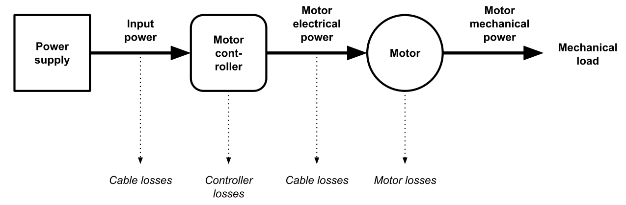
Power conversion train

While the DC input power and the mechanical output power follow the trivial relation of \(u_\text{dc} \, i_\text{dc} \approx \omega \, \tau\), the AC power transferred between the motor controller and the motor is complex as it has active and reactive components. The magnitude of the complex power (i.e., the total power, or the vector sum of the active and reactive power) for a balanced three-phase system is simply \(S = 3 \, u_\text{RMS} \, i_\text{RMS}\). The active power is dependent on the phase angle between the voltage and the current as \(P = S \, \cos{(\arg{u}-\arg{i})}\). The reactive component contributes to the losses between the motor controller and the motor but it is not manifested outside of the AC segment of the power train, hence it is not reviewed here.

In the context of a vector control drive, it is convenient to express the active power in terms of the \(dq\) system rather than relying on the generalized definition introduced earlier: \(P = \frac{3}{2} \left( u_q \, i_q + u_d \, i_d \right)\). The additional \(\frac{3}{2}\) factor is due to the fact that the \(\alpha\beta\)-transformation is not power-invariant. Assuming \(i_d \approx 0\) which holds in simple scenarios (without MTPA nor flux weakening), the expression degenerates to \(P \approx \frac{3}{2} u_q \, i_q\). (n.b.: the reactive power expressed in the \(dq\) frame is \(Q = \frac{3}{2} \left( u_q \, i_d - u_d \, i_q \right)\)). The resulting power balance equation for an electric power train is (assuming negligible losses):

\[ P_\text{dc} = u_\text{dc} \, i_\text{dc} \approx \frac{3}{2} \left( u_q \, i_q + u_d \, i_d \right) \approx \omega \, \tau = P_\text{mechanical} \]

In the case of a generator or a motor in the regenerative braking mode, we have \(\text{sgn}(\tau) \neq \text{sgn}(\omega); i_q < 0; i_\text{dc} < 0\).

Observe that the relation between the DC power and the \(dq\)-frame quantities closely resembles the power balance of a DC-DC converter: \(u_\text{in} \, i_\text{in} \approx u_\text{out} \, i_\text{out}\).

The power transfer equation is useful for choosing the drive parameters for given mechanical load requirements \(\omega, \tau\). Said requirements are often specified for multiple operating points of interest (e.g., maximum velocity, maximum torque points), in which case, the assessment is to be performed multiple times and the resulting envelope is then used to derive the drive parameters (such as the DC-link voltage and current limits). As can be seen from the motor state equations introduced earlier, the flux linkage \(\phi\) and the number of rotor poles \(p\) (n.b. the standard motor velocity constant \(K_V\) incorporates both) are the main parameters that define the relation between the voltage and the current under some constant \(\omega,\tau\). In the case of separately excited motors, one needs to consider the rotor excitation current, as it defines the rotor flux.

For the purposes of a high-level assessment of a power train, assuming optimal control outside of the flux-weakening region, one can rely on the simplified torque equation: \(\tau = \frac{3}{2} \frac{p}{2} \phi |i_{dq}|\). Solving for the current vector magnitude (i.e., phase current amplitude) yields \(|i_{dq}| = \frac{4 \, \tau}{3 \, p \, \phi}\). Assuming zero D-axis current (no flux weakening, no MTPA), \(|i_{dq}| = i_q, 0 = i_d\). From the motor state equations, assuming steady-state conditions, the \(u_{dq}\) voltage vector is obtained as:

\[\begin{split} \begin{align} u_d &= -\frac{p}{2} \omega \, L_q \, |i_{dq}| \\ u_q &= R_s |i_{dq}| + \frac{p}{2} \omega \, \phi \end{align} \end{split}\]

From the VSI voltage equation introduced earlier, we derive the minimum DC-link voltage required to produce the voltage vector as \(u_\text{dc} = \frac{\sqrt{3} |u_{dq}|}{f_\text{util}}\), where \(f_\text{util} \leq 1\) is dependent on the VSI hardware design.

The DC-link current is then derived trivially as \(i_\text{dc} = \frac{P_\text{dc}}{u_\text{dc}} = \frac{P_\text{motor}}{u_\text{dc} \, \eta}\), where \(\eta < 1\) is the expected total energy efficiency of the drive.

The final form is as follows:

\[\begin{split} \begin{align} u_\text{dc} &= \frac{ \sqrt{3} \sqrt{(\frac{2 \, L_q \, \tau \, \omega}{3 \, \phi})^2 + (\frac{4 \, \tau}{3 \, p \, \phi} R_s + \frac{p}{2} \omega \, \phi)^2} }{ f_\text{util} } \\ i_\text{dc} &= \frac{\omega \, \tau}{u_\text{dc} \, \eta} \end{align} \end{split}\]

A helper spreadsheet for drive parameter estimation is publicly available at https://docs.google.com/spreadsheets/d/1ppvrBVGf7KK1D4CLZyujGzjyCizrOxiNp3NwrBJYFlk.

Applicability of motor constants

When relying on the conventional motor constants \(K_v\) (velocity constant) and \(K_\tau\) (torque constant), one has to keep in mind the non-power-invariant nature of the \(\alpha\beta\)-transform and the relation between the DC link voltage and the AC voltages.

In SI, \(K_v = \frac{2 \sqrt3}{3 \, p \, \phi}\) [\(\frac{\text{radian}}{\text{volt}\times\text{second}}\)], and \(K_\tau = \frac1{K_v}\) [\(\frac{\text{newton}\times\text{meter}}{\text{ampere}}\)]. From the simplified torque equation presented above, we can formulate a similar torque constant for the \(dq\)-frame as \(k = \frac32 \frac{p}2 \phi\), then \(\tau = k \, i_q\).

Notice that \(\frac{K_\tau}{k} = \sqrt3 \frac23\), where \(\sqrt3\) follows from the relation between the DC link voltage and AC voltage, and \(\frac23\) arises from the non-power-invariant nature of the \(\alpha\beta\)-transform. It is therefore incorrect to use the standard motor torque constant with AC current values.

---

[1]

A useful article on the subject of magnetic system construction is available at https://things-in-motion.blogspot.com/2019/01/selecting-best-pole-and-slot.html; the calculation spreadsheet is at https://docs.google.com/spreadsheets/d/1AZ2w6lbniuLydnSUgLaUv4zhjWA-wICHkOnHHVaU8Mg/edit.

[2]

Alternative formulations of \(K_V\) exist; see motor constants.